Counterfactual Fairness Is Basically Demographic Parity
So be careful which one you use!
Counterfactual Fairness Is Basically Demographic Parity
I find that most research papers could use an accompanying translation into plain English. So, here’s my attempt at that for our paper on counterfactual fairness! The original paper lives here, and the supporting repository lives here.
Let’s dive in.
Demographic or statistical parity
Before we get into the meat of the paper, its important to understand two common fairness definitions. Let’s discuss demographic/statistical parity (note: you will see people using both names to mean the same thing. We’ll use statistical parity from now on, sometimes abbreviated SP ).
Statistical parity is a natural first fairness definition. Outside of the formalism, the best way to understand it is through an example. Consider the following candidate pool and accepted pool, where candidates can either be brainy smurfs or minions.
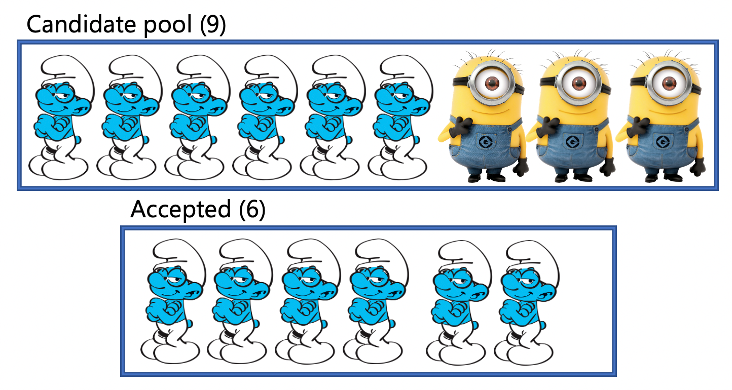
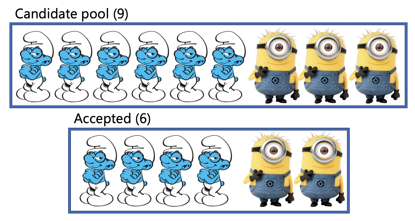
In this example, we see that the candidate pool has both brainy smurfs and minions. However, the accepted pool is 100% brainy smurfs. This would be an example of a statistical parity violation. Statistical parity is violated when the acceptance rate of a privileged group (i.e. brainy smurfs) is different than the acceptance rate of an unprivileged group (minions). Conversely, if the probability of receiving a positive label for both groups is the same, then statistical parity is satisfied. Thus, the following breakdown would satisfy statistical parity:
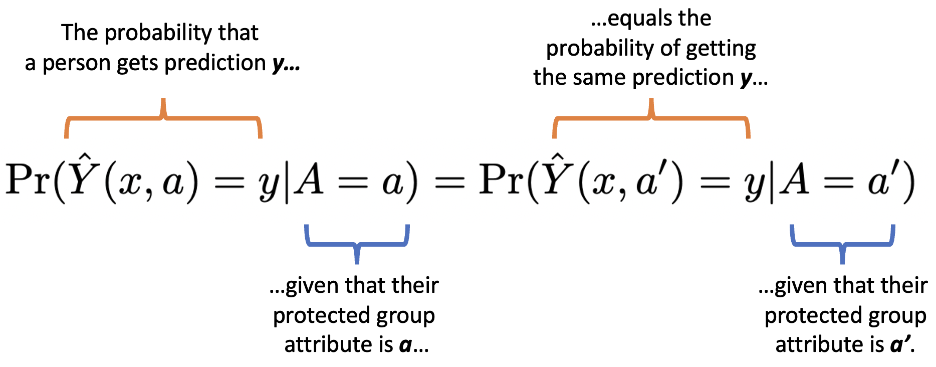
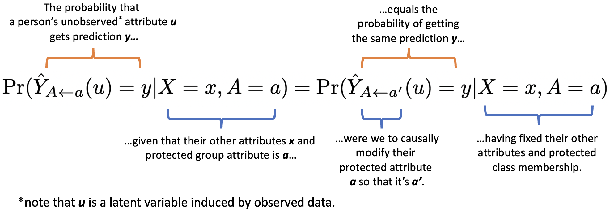
Hopefully, now the following formalism (with annotations) will make intuitive sense!
Counterfactual fairness
Let’s move on to counterfactual fairness, which appears at first a more complex fairness definition that is based on the idea of counterfactuals and causal modeling. Intuitively, a counterfactual is a statement about what would have happened had something else happened. For example, were I to say “If I had studied harder, I would have gotten an A on the test,” I would be making a counterfactual statement.
We won’t go into all of the details of causal modeling here. For a great explanation of the nuances of causal modeling and counterfactuals in particular, see this excellent blog series by Ferenc Huszár.
Instead, we will only discuss the relevant concepts to this work, again using the examples of smurfs and minions. Consider the following extremely simple structural causal model (SCM) in the smurf context:
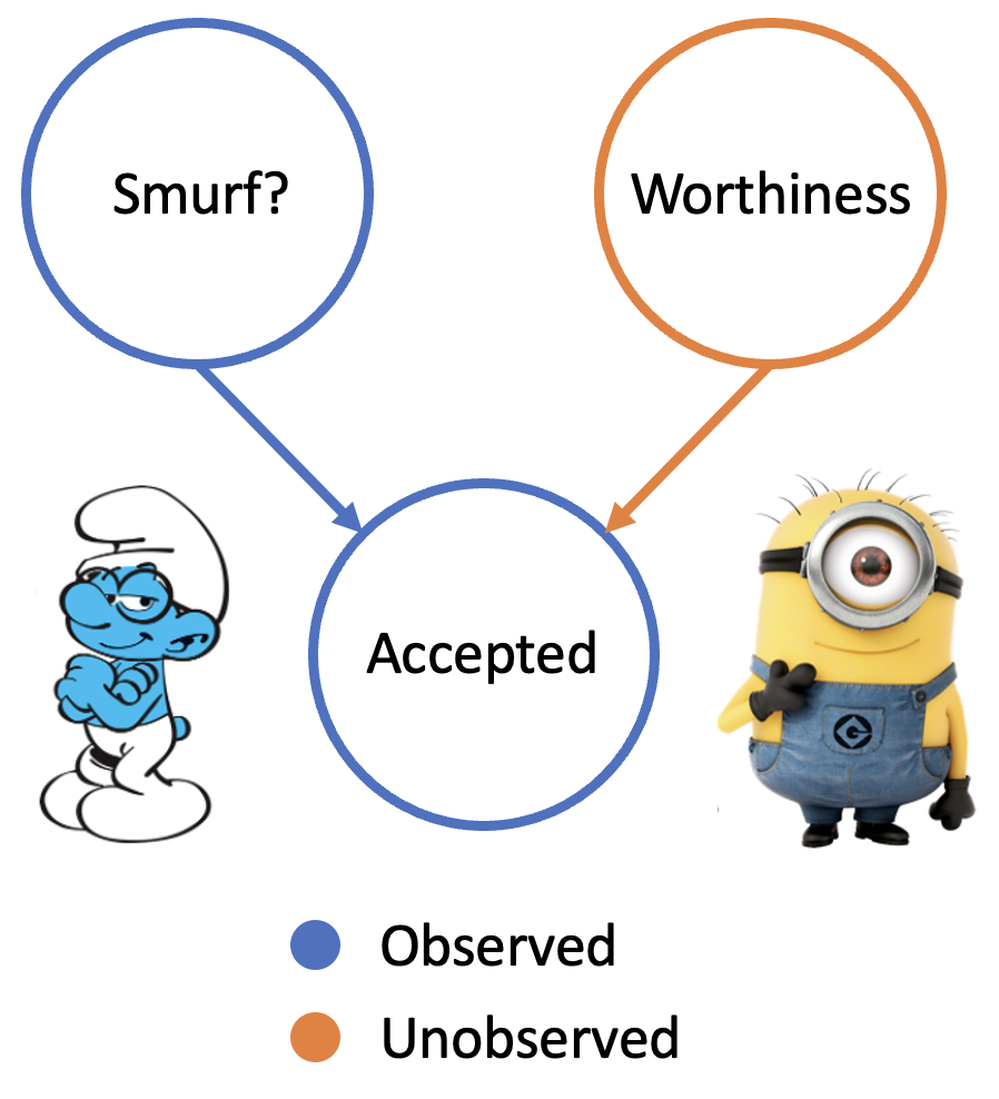
Whether a candidate gets accepted or not hinges on two factors - first, if the candidate belongs to the intellectually gifted group of brainy smurfs, and second, a latent variable known as “worthiness.”
What's a latent variable?
A "latent variable" is just a fancy name for a variable that we did not measure (i.e. we have no data on) but instead postulate as affecting our system. Using our SCM, we can infer a value for our latent variable by leveraging a mathematical model relating other variables that we did observe to our latent variable. There are many ways to do this! We do it like this, see full implementation for all details :def inferU(GroundTruthModel, data, X, latent='K'):
data = data.copy().reset_index()
# hold all K values
U=[]
for i in range(len(data)):
dictionary = {key:0 for key in X}
for key in X: dictionary[key] = torch.tensor(data[key][i])
conditioned = pyro.condition(GroundTruthModel, data=dictionary)
# use pyro.infer.Importance
posterior = pyro.infer.Importance(conditioned, num_samples=10).run()
post_marginal = pyro.infer.EmpiricalMarginal(posterior, latent)
post_samples = [post_marginal().item() for _ in range(10)]
# calculate the mean of the inferred
U += [np.mean(post_samples)]
return UThe arrows provide the causal relationships. So, in our model, Smurf? causally influences Accepted, as does Worthiness.
At this point, some of you might be scratching your heads and asking, “What about the connection between **Smurf? and Worthiness?” Well, in our model, there isn’t one!** A candidates Smurf?-ness and their Worthiness are independent of each other. In our paper, we denote this requirement as Criteria 3. But why is this a criteria?
Well, as you are hopefully beginning to understand, counterfactual fairness attempts to explain behavior from protected attributes and latent variables. The protected attributes could hold information on features outside of individuals’ control which would very often be unfair to base decisions on, while the latent variables contain information on features within an individual’s control which are fair to base decisions on. From this perspective, it is clear that in many contexts the latent variables must be independent of protected attributes. Otherwise, this would imply that, for example, the inherent ‘worthiness’ of latent variables could problematically depend on a protected attribute.
Doing a counterfactual
So, what happens if we shake things up a bit? What if we magically turned a Minion into a Brainy Smurf? This is where Judea Pearl’s “do” calculus comes in. Pearl’s “do” operator (think of it as a magic wand) lets us tweak one variable in our model and see how that changes the outcome.
With our magic wand, we could ask, “What’s the likelihood of a candidate getting accepted if we transform them into a Brainy Smurf?” This is represented as:
\[P(Acceptance = yes~|~do(Species = Brainy Smurf))\]or as
\[P(Acceptance_{Species \leftarrow Brainy Smurf} = yes)\]In other words, this tells us the probability of acceptance when we intervene and set the ‘Species’ variable to Brainy Smurf, bypassing the natural course of the universe.
This brings us to the heart of counterfactual fairness. Let’s say a Minion was accepted. Now we can ask a counterfactual question: “What if that Minion had been a Brainy Smurf? Would they still have been accepted?” By considering both our structural model and this observed data, we can dive into these alternative realities, enabling a fair comparison across different groups.
In essence, counterfactual fairness allows us to imagine an equal playing field, providing a lens to understand and measure fairness in our decisions. It challenges us to ask, “What would have happened if things were different?”, ultimately pushing us to build more just and equitable systems.
Formally, we say something like this:
So, counterfactual fairness is basically statistical parity?
How do we go about seeing this? The derivation is subtle, but short, so I’ll include it here for those who are interested.
Remember Criteria 3, it’ll come in handy in the following derivation!
Note that a predictor which satisfies counterfactual fairness must have an internal method of estimating latent variables and a causal model. So to say that a predictor which satisfies demographic parity also satisfies counterfactual fairness, we must introduce such a method and causal model. We do so in the proof of the first theorem in a trivial way.
Theorem: Any predictor $\hat{Y}': X \times A \rightarrow Y$ that satisfies demographic parity can be modified into a method for estimating latent variables and a predictor $\hat{Y}: U \times A \rightarrow Y$ that is counterfactually fair.
Proof: Our estimate of the latent variables $u$, given protected attributes $a$ and remaining attributes $x$, is $u = \hat{Y}'(x, a)$. Then the predictor $\hat{Y}: U \times A \rightarrow Y$ is given by the identity function $\hat{Y}_{A \gets a}(u) = u$. Because $\hat{Y}'$ satisfies demographic parity, we know $\Pr(u |a) = \Pr(u | a')$ for $a, a' \in A$. That is, latent variables are independent of protected attributes which meets Criteria 3. Further, $\hat{Y}$ satisfies counterfactual fairness because $\hat{Y}_{A \gets a}(u) = u = \hat{Y}_{A \gets a'}(u)$.Next we prove the converse so that we can make such a bold claim; namely, that any counterfactually fair predictor also satisfies demographic parity.